21.12.18 회귀분석
2021. 12. 19. 20:49ㆍ작업/머신러닝
실습1 기울기와 절편
# 실습에 필요한 패키지입니다. 수정하지 마세요.
import elice_utils
import matplotlib as mpl
mpl.use("Agg")
import matplotlib.pyplot as plt
import numpy as np
eu = elice_utils.EliceUtils()

# 실습에 필요한 데이터입니다. 수정하지마세요.
X = [8.70153760, 3.90825773, 1.89362433, 3.28730045, 7.39333004, 2.98984649, 2.25757240, 9.84450732, 9.94589513, 5.48321616]
Y = [5.64413093, 3.75876583, 3.87233310, 4.40990425, 6.43845020, 4.02827829, 2.26105955, 7.15768995, 6.29097441, 5.19692852]

'''
beta_0과 beta_1 을 변경하면서 그래프에 표시되는 선을 확인해 봅니다.
기울기와 절편의 의미를 이해합니다.
'''

beta_0 = 0.5   # beta_0에 저장된 기울기 값을 조정해보세요.
beta_1 = 2 # beta_1에 저장된 절편 값을 조정해보세요.

plt.scatter(X, Y) # (x, y) 점을 그립니다.
plt.plot([0, 10], [beta_1, 10 * beta_0 + beta_1], c='r') # y = beta_0 * x + beta_1 에 해당하는 선을 그립니다.

plt.xlim(0, 10) # 그래프의 X축을 설정합니다.
plt.ylim(0, 10) # 그래프의 Y축을 설정합니다.

# 엘리스에 이미지를 표시합니다.
plt.savefig("test.png")
eu.send_image("test.png")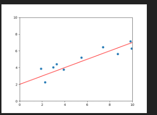
실습2 Loss function
import elice_utils
import matplotlib as mpl
mpl.use("Agg")
import matplotlib.pyplot as plt
import numpy as np
eu = elice_utils.EliceUtils()

def loss(x, y, beta_0, beta_1):
    N = len(x)

    '''
    x, y, beta_0, beta_1 을 이용해 loss값을 계산한 뒤 리턴합니다.
    '''
    total_loss = 0
    for i in range(N):
        y_i = y[i] # 실제 정답
        x_i = x[i] # 실제 input
        y_predicted = beta_0 * x_i + beta_1
        diff = (y_i - y_predicted)**2 # 편차의 제곱
        total_loss += diff
    return total_loss

X = [8.70153760, 3.90825773, 1.89362433, 3.28730045, 7.39333004, 2.98984649, 2.25757240, 9.84450732, 9.94589513, 5.48321616]
Y = [5.64413093, 3.75876583, 3.87233310, 4.40990425, 6.43845020, 4.02827829, 2.26105955, 7.15768995, 6.29097441, 5.19692852]

beta_0 = 1 # 기울기
beta_1 = 0.5 # 절편

print("Loss: %f" % loss(X, Y, beta_0, beta_1))

plt.scatter(X, Y) # (x, y) 점을 그립니다.
plt.plot([0, 10], [beta_1, 10 * beta_0 + beta_1], c='r') # y = beta_0 * x + beta_1 에 해당하는 선을 그립니다.

plt.xlim(0, 10) # 그래프의 X축을 설정합니다.
plt.ylim(0, 10) # 그래프의 Y축을 설정합니다.
plt.savefig("test.png") # 저장 후 엘리스에 이미지를 표시합니다.
eu.send_image("test.png")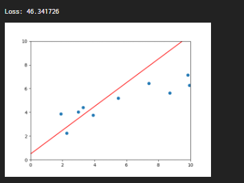
실습3 Scikit-learn을 이용한 선형회귀분석
import matplotlib as mpl
mpl.use("Agg")
import matplotlib.pyplot as plt
import numpy as np
from sklearn.linear_model import LinearRegression

import elice_utils
eu = elice_utils.EliceUtils()

def loss(x, y, beta_0, beta_1):
    N = len(x)

    '''
    이전 실습에서 구현한 loss function을 여기에 붙여넣습니다.
    '''
    x = np.array(x)
    y = np.array(y)
    total_loss = np.sum((y - (beta_0 * x + beta_1)) ** 2)
    return total_loss

X = [8.70153760, 3.90825773, 1.89362433, 3.28730045, 7.39333004, 2.98984649, 2.25757240, 9.84450732, 9.94589513, 5.48321616]
Y = [5.64413093, 3.75876583, 3.87233310, 4.40990425, 6.43845020, 4.02827829, 2.26105955, 7.15768995, 6.29097441, 5.19692852]

print(X)
train_X = np.array(X).reshape(-1,1) # 세로로 긴 array
train_Y = np.array(Y).reshape(-1,1)
print(train_X)
'''
여기에서 모델을 트레이닝합니다.
'''
lrmodel = LinearRegression() # 위에 sklearn.linear_model 에서 import 한 함수
lrmodel.fit(train_X, train_Y)

'''
loss가 최소가 되는 직선의 기울기와 절편을 계산함
'''
beta_0 = lrmodel.coef_[0]   # lrmodel로 구한 직선의 기울기
beta_1 = lrmodel.intercept_ # lrmodel로 구한 직선의 y절편

print("beta_0: %f" % beta_0)
print("beta_1: %f" % beta_1)
print("Loss: %f" % loss(X, Y, beta_0, beta_1))

plt.scatter(X, Y) # (x, y) 점을 그립니다.
plt.plot([0, 10], [beta_1, 10 * beta_0 + beta_1], c='r') # y = beta_0 * x + beta_1 에 해당하는 선을 그립니다.

plt.xlim(0, 10) # 그래프의 X축을 설정합니다.
plt.ylim(0, 10) # 그래프의 Y축을 설정합니다.
plt.savefig("test.png") # 저장 후 엘리스에 이미지를 표시합니다.
eu.send_image("test.png")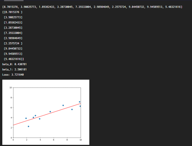
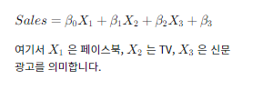
실습4 다중 회귀 분석
import numpy as np
from sklearn.linear_model import LinearRegression
from sklearn.metrics import r2_score
'''
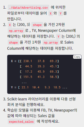
./data/Advertising.csv 에서 데이터를 읽어, X와 Y를 만듭니다.
X는 (200, 3) 의 shape을 가진 2차원 np.array,
Y는 (200,) 의 shape을 가진 1차원 np.array여야 합니다.
X는 FB, TV, Newspaper column 에 해당하는 데이터를 저장해야 합니다.
Y는 Sales column 에 해당하는 데이터를 저장해야 합니다.
'''
import csv
csvreader = csv.reader(open("data/Advertising.csv"))
x = []
y = []
next(csvreader) # 맨 첫줄 건너뛰기
for line in csvreader : # line: index, x1, x2, x3, y
print(line)
x_i = [ float(line[1]), float(line[2]), float(line[3]) ]
y_i = float(line[4])
x.append(x_i)
y.append(y_i)
X = np.array(x)
Y = np.array(y)
print(X)
print(Y)
lrmodel = LinearRegression()
lrmodel.fit(X, Y)
beta_0 = lrmodel.coef_[0] # 0번째 변수에 대한 계수 (페이스북)
beta_1 = lrmodel.coef_[1] # 1번째 변수에 대한 계수 (TV)
beta_2 = lrmodel.coef_[2] # 2번째 변수에 대한 계수 (신문)
beta_3 = lrmodel.intercept_ # y절편 (기본 판매량)
print("beta_0: %f" % beta_0)
print("beta_1: %f" % beta_1)
print("beta_2: %f" % beta_2)
print("beta_3: %f" % beta_3)
def expected_sales(fb, tv, newspaper, beta_0, beta_1, beta_2, beta_3):
'''
FB에 fb만큼, TV에 tv만큼, Newspaper에 newspaper 만큼의 광고비를 사용했고,
트레이닝된 모델의 weight 들이 beta_0, beta_1, beta_2, beta_3 일 때
예상되는 Sales 의 양을 출력합니다.
'''
sales = beta_0 * fb + beta_1 * tv + beta_2 * newspaper + beta_3
return sales
print("예상 판매량: %f" % expected_sales(10, 12, 3, beta_0, beta_1, beta_2, beta_3))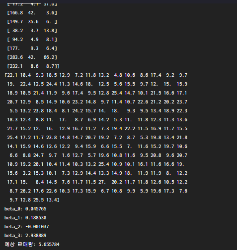
'작업 > 머신러닝' 카테고리의 다른 글
| 21.12.19 모의테스트 (0) | 2021.12.19 |
|---|---|
| 21.12.18 나이브베이즈 분류 (0) | 2021.12.19 |
| 21.12.18 선형대수 / Numpy (0) | 2021.12.19 |
| 21.12.18 머신러닝 분류(Classification) (0) | 2021.12.19 |
| 21.12.18 머신러닝 회귀(Regression) (0) | 2021.12.19 |