2022. 3. 11. 14:03ㆍ카테고리 없음
코치님 말씀
- 논문리뷰 할 때 Fig1, Fig2 먼저 보고, Abstract랑 Conclusion(실험) 만 보고 문제점과 기존연구와의 차이점?이 어떤지 먼저 파악해봐라
- ResNet을 보는 이유 : 현재에도 ResNet(2015년꺼)을 많이 사용하기 때문이다.
- ResNet: VGG 19가 19층에서 더 늘리지 못하고 있었다. 깊어질수록 학습이 잘 안되고 안좋아졌기 때문이다. 왜냐면 깊어질수록 원본 정보를 까먹게 된다. 또 추가적인 문제는 Back propagation 이기 때문에 layer가 적을 때는 back propagation 하기가 쉬운데(경우의 수가 적은데), layer가 많으면 거슬러올라가기가 힘들다. 그래서 이전 정보를 한번 더 주는(그림에서 2layer씩 뛰어넘는 것) shortcut 를 주면 layer가 깊어져도 거슬러올라가기가 쉽다.(예를들어 2layer씩 뛰어넘으면 거슬러올라가야 할 게 1/2배로 줄어든다)
- Back propagation : 예를 들어 사과이미지를 넣으면 layer를 타고 내려가면서(forward) 사과를 맞추는 게 모델의 일이다. 근데 back propagation은 거슬러 올라가는 것이다. 그런데 예를들어 결과가 배가 나온 것이다. 근데 우리는 label(정답)이 사과인 걸 안다. 그래서 배 와 사과의 차이 = loss 를 구하고, loss를 줄여나가기 위해 예측을 거슬러올라가서 제일 적은 cost(loss)를 찾아가는 것이다.
A가 아니라 B로 예측했어야했을 거 같아, C가 아니라 D였어야할 것 같아. 이런식으로 한번 거슬러올라가면
모델이 한번 바뀌고, 그럼 또 forward로 내려가서 loss를 구하고 또 backpropagation으로 거슬러 올라가면서 학습해나간다.
- 3x3 filter(conv layer)를 쓰는 이유 : 대부분 3x3이 특징을 잘 잡아내서 3x3을 쓴다. 그런데 ResNet 50부터는 3x3,1x1,3x3,1x1을 번갈아가면서 쓴다. 왜냐하면 1x1을 거치면 차원을 줄여주기 때문에(BottleNeck 구조) 레이어가 깊어도(19->50) 자원이 적어진다.
- ResNet 중에서는 ResNet50이 가장 성능이 좋아서 다들 많이 사용한다.
- 논문을 읽을 때는 main idea를 찾는 것이 중요하다.
- 모델을 코드로 구현 : torchvisions.model (https://pytorch.org/vision/stable/models.html)을 사용하면 GitHub 클론 안해도 유명한 모델들은 불러올 수 있다.
하나씩 하나씩 학습을 해보자. 어떤 하이퍼파라미터 바꿨더니 기존보다 정확도가 더 높아졌어! 만 GitHub에 잘 적어도 취업시에 많은 도움이 된다. pytorch의 Finetuning 튜토리얼 보면서 성능 업그레이드 해보는 게 중요하다.
- 학습할 때는 CIFAR 10이 학습이 빠르게 된다. 나동빈 유튜브 보면서 직접 학습을 해봐라.
- 경력기술서 : 내가 한 것들 모두 적기, 포트폴리오 : 내가 가장 주력으로 하는 것 1~3개 자세히
- 원하는 기업 잡플레닛 검색해보기, 스타트업이면 the vc도 보기(시리즈 B이상이면 이 회사 망하진 않겠다)
잡플레닛에서 2점후반대 정도 되는데로 보기
- 링크드인 일촌
ResNet 구현 블로그 : https://deep-learning-study.tistory.com/534
[논문 구현] PyTorch로 ResNet(2015) 구현하고 학습하기
이번 포스팅에서는 PyTorch로 ResNet을 구현하고 학습까지 해보겠습니다. 논문 리뷰는 여기에서 확인하실 수 있습니다. [논문 읽기] ResNet(2015) 리뷰 이번에 읽어볼 논문은 ResNet, 'Deep Residual Learni.
deep-learning-study.tistory.com
-----------------------------------------------------------------------------------------------------------------------------------
Deep Residual Learning for Image Recognition (CVPR 2016) 과 나동빈 님의 딥러닝 논문 리뷰 참고
나동빈 님의 ResNet 짧은 논문 리뷰
ResNet의 특징 : 잔여학습을 사용했다는 점.

일반적인 CNN에서는 레이어를 깊게 쌓을 수록 error도 높아질 수 있는데, 잔여학습(ResNet)은 레이어를 깊게 쌓으면 error를 더 낮출 수 있고, 전반적인 성능을 더 높일 수 있다고 한다.
일반적으로 CNN에서 레이어가 깊어질 수록 채널 수가 많아지고 w,h는 줄어든다고 한다.(convolution을 하면 점점 줄어듬)
Conv Layer의 서로 다른 filter들은 특징을 추출한다.
ResNet보기 전에 다운샘플링(conv를 진행할수록 w,h는 줄고 nc는 늘어나는 것)을 보기 위해 VGG를 한번 확인해본다.
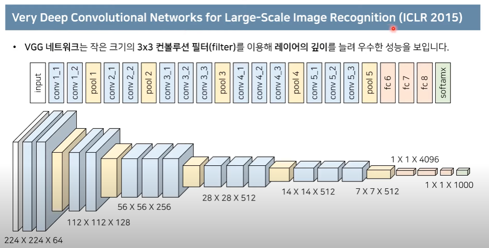
최종적으로 1000개의 class를 판별.. VGG는 layer를 깊게 줘서 성능이 좋게 나온 예시 중 하나.
그러나, 단순히 레이어를 깊게만 한다고 해서 성능이 좋아지기만 하는 것은 아님.
그런 상황에서 등장한 것이 ResNet이다
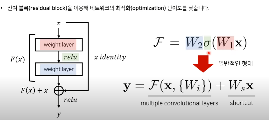
잔여 블록
ResNet에서는 레이어가 깊어지면 깊어질 수록 우리가 의도하던 대로 학습을 하기가 힘들어진다고 주장하고 있다.
즉 Conv Neural Network를 깊게 쌓기만 한다고 학습이 잘 이뤄지지 않는다.
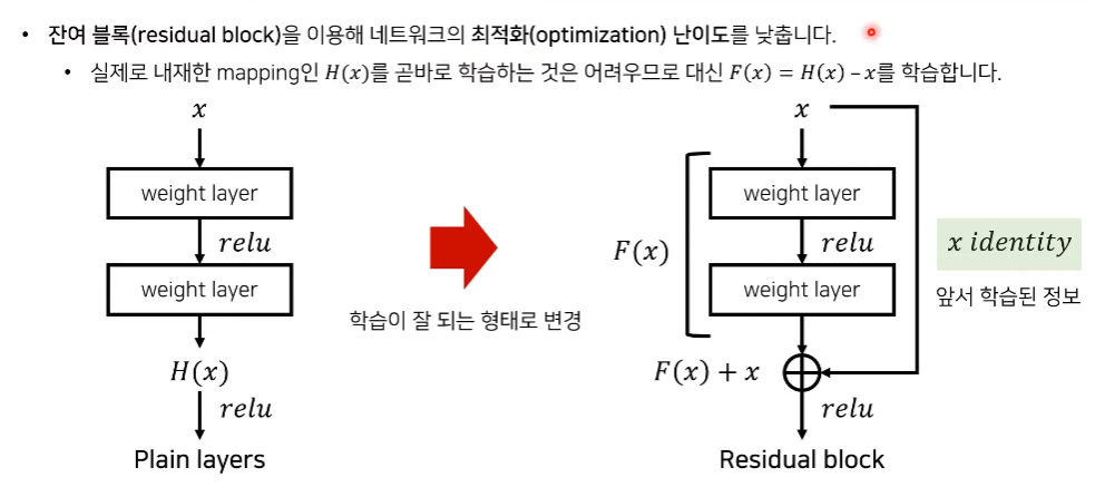
따라서 residual block이라는 것을 사용하자. 어떤 함수 H(x)를 바로 학습하기가 어려우므로 H(x)-x인 F(x)를 학습한다.
일반적 레이어(Plain layers) : weight layer(ex Conv Layer)를 거쳐서 feature를 추출한 다음 relu같은 activation을 거쳐서 non-linear한 동작을 수행할 수 있도록 해준 후 그 다음 또 Conv layer를 거친다. 이 과정을 H(x)라고 치자.
-> 수렴 난이도가 높아지고, 그 현상은 layer가 깊어질수록 더 어려워진다.
Residual Block : H(x)와 크게 바뀌지 않고 저렇게 x를 더해주는 동작 하나만 더 더하는 과정. 이 x를 더하는 과정을 하면 앞선 layer에서 학습된 정보를 그대로 가져오고, 거기에 추가적으로 잔여정보(=F(x) 동작)만 더해주면 된다.
즉, 앞선 layer에서 학습된 정보 + 추가 학습 정보(=H(x)) 를 전부 학습하는 것보다 F(x)만 학습하는 게 더 쉽다는 것
이렇게 해서 저 F(x) + x = 최종적으로 H(x)가 되도록 학습
수식으로 자세히 확인
ImageNet에서의 테스트 결과 분석(ImageNet = 이미지 분류에서 유명한 데이터셋)
plain은 그냥 VGG모델, ResNet은 VGG에 residual block을 사용한 모델
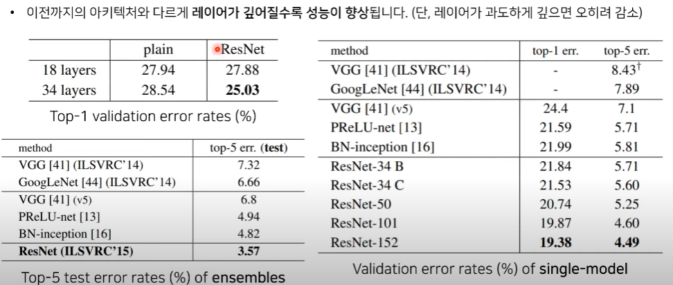
val_err 를 보면 알 수 있듯이 ResNet이 성능이 더 좋다. 추가로 앙상블(ensemble)이라는 것까지 대회에서는 적용해서 성능을 더 끌어올렸다고 한다. 앙상블을 사용하지 않은 single model에서도 성능이 더 좋다.
-----------------------------------------------------------------------------------------------------------------------------------
논문 리뷰
https://arxiv.org/abs/1512.03385
Deep Residual Learning for Image Recognition
Deeper neural networks are more difficult to train. We present a residual learning framework to ease the training of networks that are substantially deeper than those used previously. We explicitly reformulate the layers as learning residual functions with
arxiv.org
Abstract
Deeper neural networks are more difficult to train. We present a residual learning framework to ease the training of networks that are substantially deeper than those used previously. We explicitly reformulate the layers as learning residual functions with reference to the layer inputs, instead of learning unreferenced functions. We provide comprehensive empirical evidence showing that these residual networks are easier to optimize, and can gain accuracy from considerably increased depth. On the ImageNet dataset we evaluate residual nets with a depth of up to 152 layers—8× deeper than VGG nets [41] but still having lower complexity. An ensemble of these residual nets achieves 3.57% error on the ImageNet test set. This result won the 1st place on the ILSVRC 2015 classification task. We also present analysis on CIFAR-10 with 100 and 1000 layers.
The depth of representations is of central importance for many visual recognition tasks. Solely due to our extremely deep representations, we obtain a 28% relative improvement on the COCO object detection dataset. Deep residual nets are foundations of our submissions to ILSVRC & COCO 2015 competitions1 , where we also won the 1st places on the tasks of ImageNet detection, ImageNet localization, COCO detection, and COCO segmentation.
DNN은 학습시키기 어렵다. 그래서 우리는 residual learning이라는 걸 사용해서 기존에 나온 모델들보다 깊은 모델까지 학습시키기 쉽게 만들어줄 것이다. ~~ residual function은 학습이 더 잘되어서 layer를 더 깊게 해도 되고, 모델의 성능을 더 높일 수 있다.
그래서 결과적으로 ImageNet의 152 layer의 아주 깊은 ResidualNet을 평가해보았다. 이는 기존의 VGG net보다 더 깊지만 복잡도가 더 낮고(학습이 쉽고), 성능 또한 개선되었다. 그래서 이미지 분류대회 ILSVRC 2015에서 1등을 차지했다.
추가적으로 CIFAR10에 대해서도 평가해보았는데 성능이 많이 개선되었다.
깊이(Depth)는 이미지 분류 작업에서 중요한 역할을 한다. 우리의 Residual 방법은 비단 이미지분류 뿐 아니라 segmentation이나 object detection에서도 유용하게 쓰일 수 있을 것이다.
Introduction
Deep convolutional neural networks [22, 21] have led to a series of breakthroughs for image classification [21, 50, 40]. Deep networks naturally integrate low/mid/highlevel features [50] and classifiers in an end-to-end multilayer fashion, and the “levels” of features can be enriched by the number of stacked layers (depth). Recent evidence [41, 44] reveals that network depth is of crucial importance, and the leading results [41, 44, 13, 16] on the challenging ImageNet dataset [36] all exploit “very deep” [41] models, with a depth of sixteen [41] to thirty [16]. Many other nontrivial visual recognition tasks [8, 12, 7, 32, 27] have also greatly benefited from very deep models.
깊은 CNN은 이미지 분류 task에서 중요한 돌파구가 되어왔다. 깊은 NN은 low, mid, high 레벨의 feature가 뽑히고, 레이어가 깊다는 것은 저 feature들의 '레벨' 또한 풍부해질 수 있다는 뜻이고, 여러 타 논문에서도 모델의 깊이는 visual recognition task에서 중요한 역할을 한다.
Driven by the significance of depth, a question arises: Is learning better networks as easy as stacking more layers? An obstacle to answering this question was the notorious problem of vanishing/exploding gradients [1, 9], which hamper convergence from the beginning. This problem, however, has been largely addressed by normalized initialization [23, 9, 37, 13] and intermediate normalization layers [16], which enable networks with tens of layers to start converging for stochastic gradient descent (SGD) with backpropagation [22].
그럼 우린 한 가지 질문이 생기는데, 단순히 레이어만 깊게 쌓으면 더 좋은 모델이 되는 걸까? 아니다. layer를 깊게 쌓으면 vanishing gradient(레이어가 깊을 때 기울기가 0에 가까워져서 학습이 안됨)같은 문제가 생긴다. 이 문제를 해결하기 위한 해결법으로는 네트워크의 가중치값들을 초기에 적절히 초기화를 해놓아서 학습이 잘 되도록 만들자는 아이디어(normalized initialization)이다.
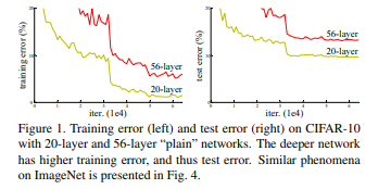
When deeper networks are able to start converging, a degradation problem has been exposed: with the network depth increasing, accuracy gets saturated (which might be unsurprising) and then degrades rapidly. Unexpectedly, such degradation is not caused by overfitting, and adding more layers to a suitably deep model leads to higher training error, as reported in [11, 42] and thoroughly verified by our experiments. Fig. 1 shows a typical example.
깊은 네트워크는 degradation problem가 발생할 수 있다. 레이어가 너무 깊으면 오히려 정확도가 감소할 수 있다. 이러한 문제는 단순히 overfitting(레이어가 깊을 때)때문만은 아니며, 너무 깊은 모델은 training error가 높아질 수 있다.
The degradation (of training accuracy) indicates that not all systems are similarly easy to optimize. Let us consider a shallower architecture and its deeper counterpart that adds more layers onto it. There exists a solution by construction to the deeper model: the added layers are identity mapping, and the other layers are copied from the learned shallower model. The existence of this constructed solution indicates that a deeper model should produce no higher training error than its shallower counterpart. But experiments show that our current solvers on hand are unable to find solutions that are comparably good or better than the constructed solution (or unable to do so in feasible time).
이런 degradation problem이 말하는 것은, 모든 모델이 학습이 다 잘된다는 것은 아니다. 우리가 한 가지 생각해볼 수 있는 건 그럼 레이어를 깊게 쌓기 위해서는 단순히 identity mapping만 증가시키면 되지 않을까? 하는 생각이 들 수 있다.
깊은 모델이 얕은 모델에 identity mapping만 추가시킨 모델에 비해 더 높은 training error를 가지는 것이 말이 안된다?
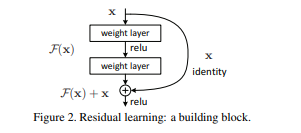
In this paper, we address the degradation problem by introducing a deep residual learning framework. Instead of hoping each few stacked layers directly fit a desired underlying mapping, we explicitly let these layers fit a residual mapping. Formally, denoting the desired underlying mapping as H(x), we let the stacked nonlinear layers fit another mapping of F(x) := H(x)−x. The original mapping is recast into F(x)+x. We hypothesize that it is easier to optimize the residual mapping than to optimize the original, unreferenced mapping. To the extreme, if an identity mapping were optimal, it would be easier to push the residual to zero than to fit an identity mapping by a stack of nonlinear layers.
그래서 우리는~~ 이 논문에서 deep residual learning framework를 제안한다. 우리가 의도했던 mapping H(x)를 바로 학습해버리기보다는 더 학습하기 쉬운 residual mapping인 F(x) = H(x)-x를 학습하겠다는 것이다. ~~ 극단적으로 생각해봤을 때 만약 identity mapping이 optimal한 해라고 했을 때 F(x)가 0이 되는 게 제일 쉽지 않겠냐? 즉 H(x)가 x가 되는 게 제일 쉽다?
The formulation of F(x) +x can be realized by feedforward neural networks with “shortcut connections” (Fig. 2). Shortcut connections [2, 34, 49] are those skipping one or more layers. In our case, the shortcut connections simply perform identity mapping, and their outputs are added to the outputs of the stacked layers (Fig. 2). Identity shortcut connections add neither extra parameter nor computational complexity. The entire network can still be trained end-to-end by SGD with backpropagation, and can be easily implemented using common libraries (e.g., Caffe [19]) without modifying the solvers.
따라서 그냥 F(x) 에 x를 더한 F(x) + x를 shortcut connection으로 사용하고 얘는 별도의 파라미터나 계산이 필요 없다.
We present comprehensive experiments on ImageNet [36] to show the degradation problem and evaluate our method. We show that: 1) Our extremely deep residual nets are easy to optimize, but the counterpart “plain” nets (that simply stack layers) exhibit higher training error when the depth increases; 2) Our deep residual nets can easily enjoy accuracy gains from greatly increased depth, producing results substantially better than previous networks. Similar phenomena are also shown on the CIFAR-10 set [20], suggesting that the optimization difficulties and the effects of our method are not just akin to a particular dataset. We present successfully trained models on this dataset with over 100 layers, and explore models with over 1000 layers.
그래서 학습하기가 쉽다~ ResNet같은 경우는 깊이가 깊어질수록 더 높은 accuracy를 보였다는 장점이 있다. 또한 ImageNet뿐 아니라 CIFAR에서도 증명되었으므로 특정 데이터셋에 국한되지 않을 것이다~
On the ImageNet classification dataset [36], we obtain excellent results by extremely deep residual nets. Our 152- layer residual net is the deepest network ever presented on ImageNet, while still having lower complexity than VGG nets [41]. Our ensemble has 3.57% top-5 error on the ImageNet test set, and won the 1st place in the ILSVRC 2015 classification competition. The extremely deep representations also have excellent generalization performance on other recognition tasks, and lead us to further win the 1st places on: ImageNet detection, ImageNet localization, COCO detection, and COCO segmentation in ILSVRC & COCO 2015 competitions. This strong evidence shows that the residual learning principle is generic, and we expect that it is applicable in other vision and non-vision problems.
여기에 금상첨화로 앙상블(ensemble)까지 적용하면 4% 안 에러로 좋은 accuracy를 뽑아낸다~
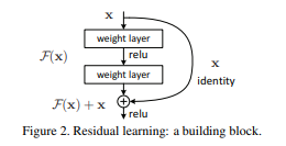
ResNet을 사용하면 우리는 H(x)대신 요 F(x)만 학습하면 되고, 그게 더 쉽다.
Related Work
Deep Residual Learning
Let us consider H(x) as an underlying mapping to be fit by a few stacked layers (not necessarily the entire net), with x denoting the inputs to the first of these layers. If one hypothesizes that multiple nonlinear layers can asymptotically approximate complicated functions2 , then it is equivalent to hypothesize that they can asymptotically approximate the residual functions, i.e., H(x) − x (assuming that the input and output are of the same dimensions). So rather than expect stacked layers to approximate H(x), we explicitly let these layers approximate a residual function F(x) := H(x) − x. The original function thus becomes F(x)+x. Although both forms should be able to asymptotically approximate the desired functions (as hypothesized), the ease of learning might be different.
어려운 H(x)대신 쉬운 F(x)를 학습시킨다. 사실 H(x)나 H(x)-x나 크게 다를 게 없어보이는데 이렇게 동일한 수식이어도 방식을 바꾸어 새로운 효과를 내는 것이 잘 이해가 안갈 수 있다.
This reformulation is motivated by the counterintuitive phenomena about the degradation problem (Fig. 1, left). As we discussed in the introduction, if the added layers can be constructed as identity mappings, a deeper model should have training error no greater than its shallower counterpart. The degradation problem suggests that the solvers might have difficulties in approximating identity mappings by multiple nonlinear layers. With the residual learning reformulation, if identity mappings are optimal, the solvers may simply drive the weights of the multiple nonlinear layers toward zero to approach identity mappings.
그러나 최소한 더 깊은 모델의 training error가 더 얕은 모델의 것보다 더 커지지는 않을 것이다.
In real cases, it is unlikely that identity mappings are optimal, but our reformulation may help to precondition the problem. If the optimal function is closer to an identity mapping than to a zero mapping, it should be easier for the solver to find the perturbations with reference to an identity mapping, than to learn the function as a new one. We show by experiments (Fig. 7) that the learned residual functions in general have small responses, suggesting that identity mappings provide reasonable preconditioning.
물론 실제로는 identity mapping이 optimal할 경우는 희박하다. 그럼에도 불구하고 이런 mapping을 추가해주는 것 자체가 딥러닝을 쉽게 할 수 있도록 해주는 방법이라는 것이다. ~~ 정리하자면 이전 layer에서 온 값인 x는 보존하고, 추가적인(residual) 정보만 학습하는 게 더 쉽다. (매번 새로운 함수를 학습시키는 것보단 쉽다.)
We adopt residual learning to every few stacked layers. A building block is shown in Fig. 2. Formally, in this paper we consider a building block defined as: y = F(x, {Wi}) + x.
여기서 F(x, {Wi})는 residual mapping이고 x는 identity mapping(shortcut connection)이다.
또한 만약 W가 한 개만 있다면(깊은 레이어는 W1,W2,W3..가는데 W1만 있는 경우)는 크게 advantage가 없다.
Here x and y are the input and output vectors of the layers considered. The function F(x, {Wi}) represents the residual mapping to be learned. For the example in Fig. 2 that has two layers, F = W2σ(W1x) in which σ denotes ReLU [29] and the biases are omitted for simplifying notations. The operation F + x is performed by a shortcut connection and element-wise addition. We adopt the second nonlinearity after the addition (i.e., σ(y), see Fig. 2).
그리고 plain 모델은 F = W2σ(W1x)로 쓴다.
The dimensions of x and F must be equal in Eqn.(1). If this is not the case (e.g., when changing the input/output channels), we can perform a linear projection Ws by the shortcut connections to match the dimensions: y = F(x, {Wi}) + Wsx.
그리고 만약 F와 x가 dimension이 맞지 않으면 Ws를 linear projection을 해줘서 dimension또한 맞춰줄 수 있다~
Plain Network. Our plain baselines (Fig. 3, middle) are mainly inspired by the philosophy of VGG nets [41] (Fig. 3, left). The convolutional layers mostly have 3×3 filters and follow two simple design rules: (i) for the same output feature map size, the layers have the same number of filters; and (ii) if the feature map size is halved, the number of filters is doubled so as to preserve the time complexity per layer. We perform downsampling directly by convolutional layers that have a stride of 2. The network ends with a global average pooling layer and a 1000-way fully-connected layer with softmax. The total number of weighted layers is 34 in Fig. 3 (middle).
plain 네트워크는 VGG를 따른다. 필터는 3x3을 사용했고, filter갯수는 동일하게 했고, 다운샘플링도 진행했고.. 총 1000개의 클래스를 분류하도록 했다. 모델 사용한 방법 설명하는 문단.
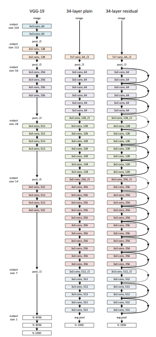
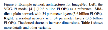
보면 residual을 적용한 것이 W1W2 두 레이어씩 묶어서 우회한 화살표로 나타나있다. 점선 화살표는 input과 output의 dimension이 맞지 않아서 dimension을 맞춰주는 2로 나눠주는 수식이 들어간 shortcut connection 부분이다.
저 보라색레이어들, 초록레이어들, 빨간레이어들, 파란레이어들이 각각 같은 색깔끼리 중첩된 레이어이다.
Residual Network. Based on the above plain network, we insert shortcut connections (Fig. 3, right) which turn the network into its counterpart residual version. The identity shortcuts (Eqn.(1)) can be directly used when the input and output are of the same dimensions (solid line shortcuts in Fig. 3). When the dimensions increase (dotted line shortcuts in Fig. 3), we consider two options: (A) The shortcut still performs identity mapping, with extra zero entries padded for increasing dimensions. This option introduces no extra parameter; (B) The projection shortcut in Eqn.(2) is used to match dimensions (done by 1×1 convolutions). For both options, when the shortcuts go across feature maps of two sizes, they are performed with a stride of 2.
입력단과 출력단의 dimension이 동일할 때는 identity mapping을 사용할 수 있고 그렇지 않으면 두 가지 옵션이 있다. 패딩을 주거나, projection shortcut connection로 진행한다.
Implementation Our implementation for ImageNet follows the practice in [21, 41]. The image is resized with its shorter side randomly sampled in [256, 480] for scale augmentation [41]. A 224×224 crop is randomly sampled from an image or its horizontal flip, with the per-pixel mean subtracted [21]. The standard color augmentation in [21] is used. We adopt batch normalization (BN) [16] right after each convolution and before activation, following [16]. We initialize the weights as in [13] and train all plain/residual nets from scratch. We use SGD with a mini-batch size of 256. The learning rate starts from 0.1 and is divided by 10 when the error plateaus, and the models are trained for up to 60 × 104 iterations. We use a weight decay of 0.0001 and a momentum of 0.9. We do not use dropout [14], following the practice in [16]. In testing, for comparison studies we adopt the standard 10-crop testing [21]. For best results, we adopt the fullyconvolutional form as in [41, 13], and average the scores at multiple scales (images are resized such that the shorter side is in {224, 256, 384, 480, 640}).
224x224로 이미지를 크롭했고, horizontal filp을 사용할 수 있다. Resnet의 경우 매 conv layer를 거칠 때마다 BN(배치정규화)를 거치도록 했고, lr는 0.1에서 시작해 점점 줄여나가는 방법을 사용했다(자주 사용되는 방법이라고 함 나동빈 님)
그리고 ~~하이퍼파라미터를 지정하여 학습을 진행했다.
ImageNet Classification We evaluate our method on the ImageNet 2012 classification dataset [36] that consists of 1000 classes. The models are trained on the 1.28 million training images, and evaluated on the 50k validation images. We also obtain a final result on the 100k test images, reported by the test server. We evaluate both top-1 and top-5 error rates.
이제 평가 진행. 우리는 1000개의 클래스가 있는 ImageNet 2012 데이터셋을 사용했다. training images는 128만개, val는 5만개정도 있다.
Plain Networks. We first evaluate 18-layer and 34-layer plain nets. The 34-layer plain net is in Fig. 3 (middle). The 18-layer plain net is of a similar form. See Table 1 for detailed architectures.
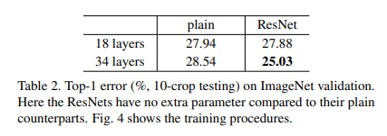
The results in Table 2 show that the deeper 34-layer plain net has higher validation error than the shallower 18-layer plain net. To reveal the reasons, in Fig. 4 (left) we compare their training/validation errors during the training procedure. We have observed the degradation problem - the 34-layer plain net has higher training error throughout the whole training procedure, even though the solution space of the 18-layer plain network is a subspace of that of the 34-layer one.
그럼 이제 비교해보자. plain 네트워크는 네트워크가 깊어질수록 얕은애보다 error가 더 올라갔다. 그런데 resnet같은 경우는 네트워크가 깊은 애가 얕은 애보다 성능도 좋고 error도 적다.
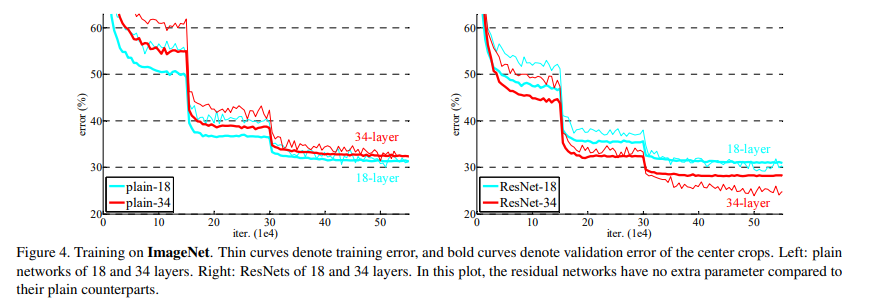
We argue that this optimization difficulty is unlikely to be caused by vanishing gradients. These plain networks are trained with BN [16], which ensures forward propagated signals to have non-zero variances. We also verify that the backward propagated gradients exhibit healthy norms with BN. So neither forward nor backward signals vanish. In fact, the 34-layer plain net is still able to achieve competitive accuracy (Table 3), suggesting that the solver works to some extent. We conjecture that the deep plain nets may have exponentially low convergence rates, which impact the reducing of the training error3 . The reason for such optimization difficulties will be studied in the future.
또한 신기한 것은 vanishing gradient문제때문에 이런 결과가 나온 것은 아니다. 실제로 우리가 학습과정에서 forward 와 backward를 확인해봤을 때 실제로 몇몇 신호가 사라지는 문제가 발생하지는 않았다. 오히려 이런 문제가 발생하는 이유는 exponentially low convergence rates 때문이다.(즉 기울기가 사라지진 않고, 기하급수적으로 낮아지는 문제?이다)
Residual Networks. Next we evaluate 18-layer and 34- layer residual nets (ResNets). The baseline architectures are the same as the above plain nets, expect that a shortcut connection is added to each pair of 3×3 filters as in Fig. 3 (right). In the first comparison (Table 2 and Fig. 4 right), we use identity mapping for all shortcuts and zero-padding for increasing dimensions (option A). So they have no extra parameter compared to the plain counterparts. We have three major observations from Table 2 and Fig. 4. First, the situation is reversed with residual learning – the 34-layer ResNet is better than the 18-layer ResNet (by 2.8%). More importantly, the 34-layer ResNet exhibits considerably lower training error and is generalizable to the validation data. This indicates that the degradation problem is well addressed in this setting and we manage to obtain accuracy gains from increased depth.
Second, compared to its plain counterpart, the 34-layer ResNet reduces the top-1 error by 3.5% (Table 2), resulting from the successfully reduced training error (Fig. 4 right vs. left). This comparison verifies the effectiveness of residual learning on extremely deep systems. Last, we also note that the 18-layer plain/residual nets are comparably accurate (Table 2), but the 18-layer ResNet converges faster (Fig. 4 right vs. left). When the net is “not overly deep” (18 layers here), the current SGD solver is still able to find good solutions to the plain net. In this case, the ResNet eases the optimization by providing faster convergence at the early stage.
결과적으로 Residual net을 사용했을 때 더 깊은 레이어(34)가 더 얕은 레이어(18)보다 에러가 낮았으며 일반화 성능도 높다. 또한 수렴속도도 일반 모델보다 더 빨라서 optimization을 더 쉽게 만들어준다는 장점이 있다.
Identity vs. Projection Shortcuts. We have shown that parameter-free, identity shortcuts help with training. Next we investigate projection shortcuts (Eqn.(2)). In Table 3 we compare three options: (A) zero-padding shortcuts are used for increasing dimensions, and all shortcuts are parameterfree (the same as Table 2 and Fig. 4 right); (B) projection shortcuts are used for increasing dimensions, and other shortcuts are identity; and (C) all shortcuts are projections. Table 3 shows that all three options are considerably better than the plain counterpart. B is slightly better than A. We argue that this is because the zero-padded dimensions in A indeed have no residual learning. C is marginally better than B, and we attribute this to the extra parameters introduced by many (thirteen) projection shortcuts. But the small differences among A/B/C indicate that projection shortcuts are not essential for addressing the degradation problem. So we do not use option C in the rest of this paper, to reduce memory/time complexity and model sizes. Identity shortcuts are particularly important for not increasing the complexity of the bottleneck architectures that are introduced below.
또한 아까 있었던 dimension맞출 때 identity mapping을 쓸 것이냐 projection shortcut이 더 좋냐에 대한 성능비교도 추가적으로 해보았는데
(A) 제로 패딩으로 dimension 늘려주고 identity mapping 사용
(B) dimension이 증가할 때만 projection mapping사용
(C) 모든 shortcut에 대해 projection 사용
-> 이 결과 C가 가장 성능이 좋긴 했는데, projection shorcut이 degradation 문제를 해결하는데 있어서 필수적인 것은ㅇ 아니다. 기본적으로 identity shortcut을 이용해 성능을 많이 개선시킨다.
Deeper Bottleneck Architectures. Next we describe our deeper nets for ImageNet. Because of concerns on the training time that we can afford, we modify the building block as a bottleneck design4 . For each residual function F, we use a stack of 3 layers instead of 2 (Fig. 5). The three layers are 1×1, 3×3, and 1×1 convolutions, where the 1×1 layers are responsible for reducing and then increasing (restoring) dimensions, leaving the 3×3 layer a bottleneck with smaller input/output dimensions. Fig. 5 shows an example, where both designs have similar time complexity. The parameter-free identity shortcuts are particularly important for the bottleneck architectures. If the identity shortcut in Fig. 5 (right) is replaced with projection, one can show that the time complexity and model size are doubled, as the shortcut is connected to the two high-dimensional ends. So identity shortcuts lead to more efficient models for the bottleneck designs.
특히 identity shortcut은 bottleneck 구조에서는 복잡도를 줄이는 데 있어서 효율적이다. identity shortcut은 파라미터가 없기 때문에 bottleneck 구조에서 효율적인 것.
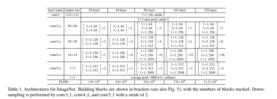
50-layer ResNet: We replace each 2-layer block in the 34-layer net with this 3-layer bottleneck block, resulting in a 50-layer ResNet (Table 1). We use option B for increasing dimensions. This model has 3.8 billion FLOPs. 101-layer and 152-layer ResNets: We construct 101- layer and 152-layer ResNets by using more 3-layer blocks (Table 1). Remarkably, although the depth is significantly increased, the 152-layer ResNet (11.3 billion FLOPs) still has lower complexity than VGG-16/19 nets (15.3/19.6 billion FLOPs). The 50/101/152-layer ResNets are more accurate than the 34-layer ones by considerable margins (Table 3 and 4). We do not observe the degradation problem and thus enjoy significant accuracy gains from considerably increased depth. The benefits of depth are witnessed for all evaluation metrics (Table 3 and 4).
따라서 34뿐 아니라 50, 100 레이어에서도 성능이 좋았지만 기존의 VGG보다 복잡도는 더 낮다는 장점이 있다.
CIFAR-10 and Analysis We conducted more studies on the CIFAR-10 dataset [20], which consists of 50k training images and 10k testing images in 10 classes. We present experiments trained on the training set and evaluated on the test set. Our focus is on the behaviors of extremely deep networks, but not on pushing the state-of-the-art results, so we intentionally use simple architectures as follows. The plain/residual architectures follow the form in Fig. 3 (middle/right). The network inputs are 32×32 images, with the per-pixel mean subtracted. The first layer is 3×3 convolutions. Then we use a stack of 6n layers with 3×3 convolutions on the feature maps of sizes {32, 16, 8} respectively, with 2n layers for each feature map size. The numbers of filters are {16, 32, 64} respectively. The subsampling is performed by convolutions with a stride of 2. The network ends with a global average pooling, a 10-way fully-connected layer, and softmax. There are totally 6n+2 stacked weighted layers. The following table summarizes the architecture:
또한 이미지넷 뿐 아니라 CIFAR-10도 평가해보았는데 일단 CIFAR는 ImageNet보다 이미지가 작다(32x32) 그래서 파라미터 수도 더 작게 했다. 그래서 첫 레이어는 3x3 conv를 진행하고.. 여러 설정을 해서 총 6n+2개의 weighted layers를 사용한다.(예를 들어 n이 3이면 20개의 layer를 사용하는 것이다.)
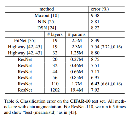
그러나 실제로는 비교대상인 original model을 VGG에서 그대로 가져다 쓰진 않는다. 보통 자기가 주장하는 Net의 #params 대비 성능이 더 잘 나오도록 적절히 조절해서 가져다 쓴다고 한다. (나동빈님의 첨언)
- 작은 데이터셋에 대해 너무 깊은 레이어를 쌓게 되면 overfitting이 생긴다.
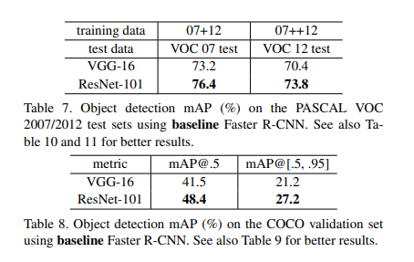
또한 object detection에서도 COCO 데이터셋과 pascal 데이터셋을 평가한 결과 ResNet의 성능이 좋게 나왔다고 한다.